What is mdgm?
The mdgm package implements Bayesian inference for discrete spatial random fields. It supports two spatial model families:
- Mixture of Directed Graphical Models (MDGM) — defines a mixture over directed acyclic graphs (DAGs) compatible with an undirected graph. Each DAG admits a tractable likelihood, avoiding the partition function entirely.
- Markov Random Field (MRF) — the classical Potts/Ising model on the same graph. Inference for the dependence parameter uses either the exchange algorithm (exact) or pseudo-likelihood (approximate).
Both can be combined with emission distributions (Bernoulli, Gaussian, Poisson) for hierarchical models where the spatial field is latent.
The MDGM approach is described in:
Carter, J. B. and Calder, C. A. (2024). Mixture of Directed Graphical Models for Discrete Spatial Random Fields. arXiv:2406.15700
Building a graph
Create a 4x4 grid graph with rook adjacency using
nug_from_grid():
nug <- nug_from_grid(4, 4, seed = 42L)
nug$nvertices()
#> [1] 16
nug$nedges()
#> [1] 24
Graphs can also be constructed from an adjacency matrix, edge list, or adjacency list — see the Working with Undirected Graphs vignette.
Visualizing the graph with igraph
The igraph package (suggested, not required) provides a quick way to visualize the neighborhood structure:
library(igraph)
#>
#> Attaching package: 'igraph'
#> The following objects are masked from 'package:stats':
#>
#>     decompose, spectrum
#> The following object is masked from 'package:base':
#>
#>     union

# Build igraph object from the NUG edge structure
n <- nug$nvertices()
el <- do.call(rbind, lapply(1:n, function(v) {
  nbrs <- nug$neighbors(v)
  nbrs <- nbrs[nbrs > v]
  if (length(nbrs) == 0) return(NULL)
  cbind(v, nbrs)
}))
g <- graph_from_edgelist(el, directed = FALSE)

# Grid layout matching the spatial positions
coords <- cbind((seq_len(n) - 1) %% 4 + 1, 4 - (seq_len(n) - 1) %/% 4)

plot(g, layout = coords, vertex.size = 20, vertex.label = 1:n,
     vertex.label.color = "white", vertex.color = "steelblue",
     edge.color = "grey40", main = "4x4 Grid Graph")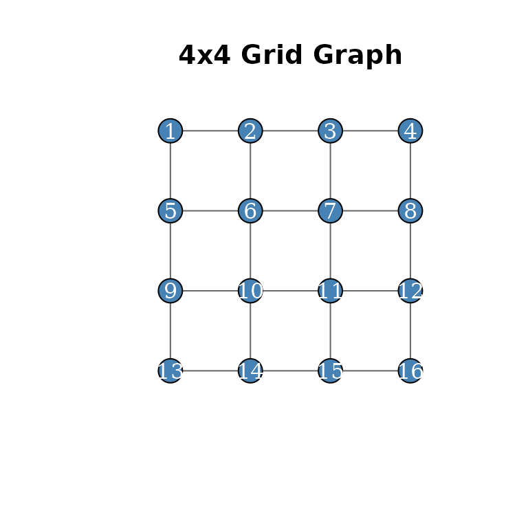
Fitting a standalone MDGM
In a standalone model, the spatial field is observed directly — no emission distribution is needed. Here we fit a spanning-tree MDGM to a deterministic checkerboard pattern on the 4x4 grid:
z <- c(0L, 0L, 0L, 1L,
       0L, 0L, 1L, 1L,
       1L, 1L, 1L, 0L,
       1L, 1L, 0L, 0L)

model <- srf_model(nug, spatial = mdgm(dag_type = "spanning_tree"))

result <- mcmc(model, z_init = z, psi_init = 0.5,
               n_iter = 2000L, psi_tune = 1.0, seed = 42L)
result$summary()
#> MDGM MCMC Results
#>   Vertices: 16, Colors: 2
#>   Iterations: 2000 (burnin: 0)
#>   Psi acceptance rate: 0.478
#>   Psi posterior mean: 0.8446 (sd: 0.5612)
#>   Diagnostics:
#>     psi — R-hat: 1.0013, ESS: 272
We can color the graph vertices by their field values:
plot(g, layout = coords, vertex.size = 20, vertex.label = 1:n,
     vertex.color = c("#440154", "#fde725")[z + 1],
     vertex.label.color = "white", edge.color = "grey40",
     main = "Spatial Field on Grid")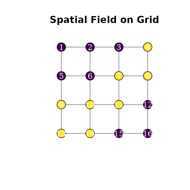
Or visualize as a raster:
grid_df <- data.frame(
  x = rep(1:4, times = 4),
  y = rep(4:1, each = 4),
  z = factor(z)
)

ggplot(grid_df, aes(x, y, fill = z)) +
  geom_raster() +
  scale_fill_manual(values = c("0" = "#440154", "1" = "#fde725")) +
  coord_equal() +
  theme_minimal() +
  labs(title = "4x4 Spatial Field", fill = "z")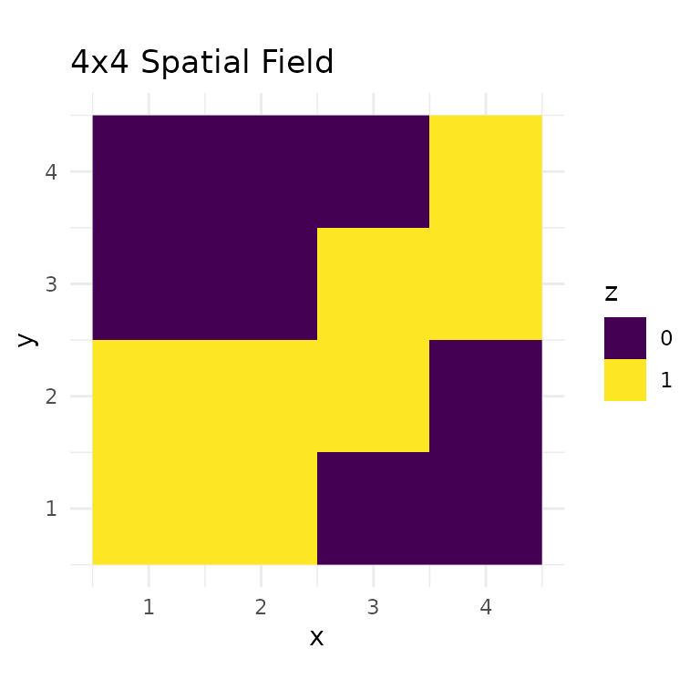
Posterior diagnostics
Trace plot for the spatial dependence parameter :
psi_df <- data.frame(iteration = seq_along(result$psi()), psi = result$psi())

ggplot(psi_df, aes(iteration, psi)) +
  geom_line(linewidth = 0.3) +
  theme_minimal() +
  labs(x = "Iteration", y = expression(psi), title = "Psi trace plot")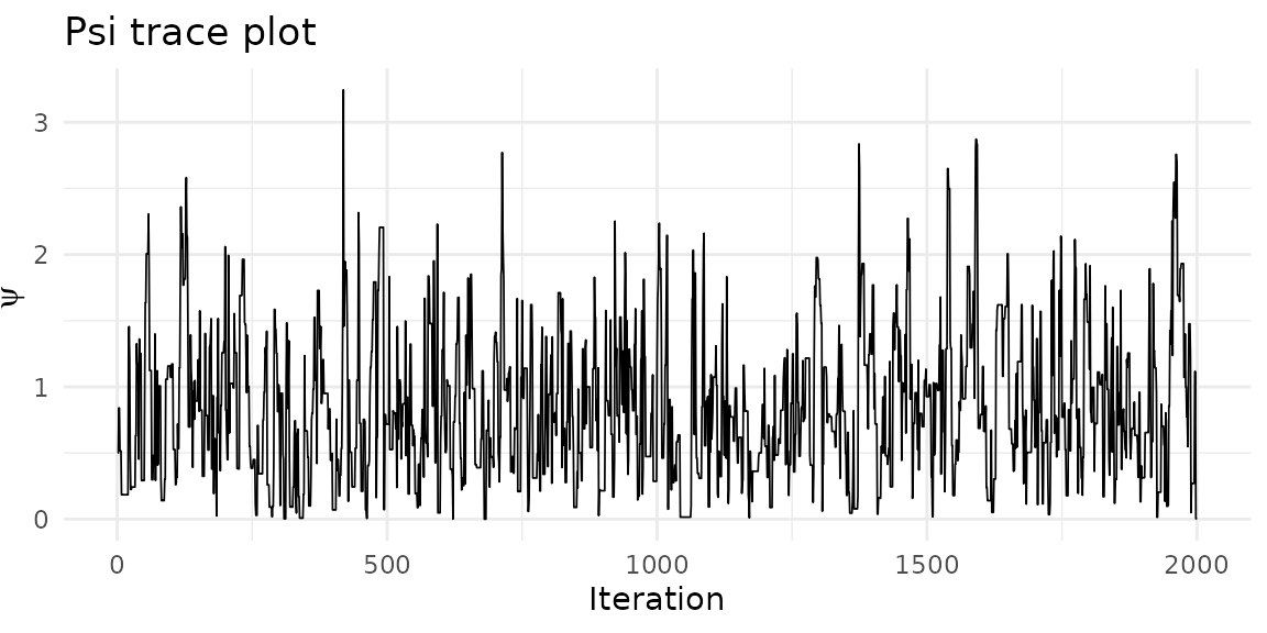
Acceptance rates:
result$acceptance_rates()
#>       psi     graph
#> 0.4777389 0.0000000
Edge inclusion probabilities
The edge_inclusion_probs() method counts how often each
undirected edge appears in the posterior spanning-tree samples. We can
use these proportions to scale edge widths:
eip <- result$edge_inclusion_probs(nug, burnin = 200L)
head(eip[order(-eip$prob), ])
#>    vertex1 vertex2      prob
#> 7        4       8 0.8116667
#> 21      12      16 0.8111111
#> 24      15      16 0.7794444
#> 3        2       3 0.7700000
#> 1        1       2 0.7238889
#> 2        1       5 0.7177778

# Match edge inclusion probs to igraph edge ordering
edge_probs <- numeric(ecount(g))
for (i in seq_len(nrow(eip))) {
  eid <- get.edge.ids(g, c(eip$vertex1[i], eip$vertex2[i]))
  edge_probs[eid] <- eip$prob[i]
}
#> Warning: `get.edge.ids()` was deprecated in igraph 2.1.0.
#> ℹ Please use `get_edge_ids()` instead.
#> This warning is displayed once per session.
#> Call `lifecycle::last_lifecycle_warnings()` to see where this warning was
#> generated.

plot(g, layout = coords, vertex.size = 20, vertex.label = 1:n,
     vertex.color = c("#440154", "#fde725")[z + 1],
     vertex.label.color = "white",
     edge.width = edge_probs * 10,
     edge.color = "grey30",
     main = "Edge inclusion probabilities")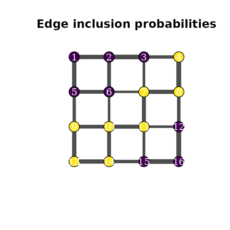
Edges between same-colored vertices appear more frequently in the posterior spanning trees, reflecting the spatial dependence captured by .
Fitting a hierarchical model
In a hierarchical model, is a latent field and observations are generated through an emission distribution. Here we use a Bernoulli emission:
model_h <- srf_model(nug, spatial = mdgm(dag_type = "spanning_tree"),
                     emission = "bernoulli")

# Simulate 5 Bernoulli observations per vertex (multiple needed for identifiability)
set.seed(1)
p_true <- c(0.2, 0.8)
y <- lapply(seq_len(n), function(i) rbinom(5, 1, p_true[z[i] + 1]))

result_h <- mcmc(model_h, y = y, z_init = sample(0:1, n, replace = TRUE),
                 psi_init = 0.5, theta_init = c(0.3, 0.7),
                 n_iter = 500L, seed = 42L)
result_h$summary()
#> MDGM MCMC Results
#>   Vertices: 16, Colors: 2
#>   Iterations: 500 (burnin: 0)
#>   Psi acceptance rate: 0.896
#>   Psi posterior mean: 0.6269 (sd: 0.5127)
#>   Emission type: bernoulli
#>   p_1 posterior mean: 0.2284 (sd: 0.0792)
#>   p_2 posterior mean: 0.8089 (sd: 0.0675)
#>   Diagnostics:
#>     psi — R-hat: 1.0124, ESS: 6
#>     p_1 — R-hat: 1.0025, ESS: 63
#>     p_2 — R-hat: 0.9989, ESS: 207
Markov random field models
The package also supports classical MRF (Potts/Ising) models on the
same graph. The mrf() configuration helper specifies the
inference method for the dependence parameter
:
-
"exchange"— the exchange algorithm, which cancels the intractable partition function by sampling an auxiliary field (exact) -
"pseudo_likelihood"— replaces the joint likelihood with the product of full conditionals (fast, approximate)
# MRF with pseudo-likelihood inference
model_mrf <- srf_model(nug, spatial = mrf(method = "pseudo_likelihood"))

result_mrf <- mcmc(model_mrf, z_init = z, psi_init = 0.5,
                   n_iter = 2000L, psi_tune = 0.5, seed = 42L)
result_mrf$summary()
#> MRF MCMC Results
#>   Vertices: 16, Colors: 2
#>   Iterations: 2000 (burnin: 0)
#>   Psi acceptance rate: 0.681
#>   Psi posterior mean: 0.8784 (sd: 0.4959)
#>   Diagnostics:
#>     psi — R-hat: 1.0057, ESS: 158
The exchange algorithm is more expensive per iteration but provides exact inference:
model_ex <- srf_model(nug, spatial = mrf(method = "exchange",
                                         n_aux_sweeps = 100L))

result_ex <- mcmc(model_ex, z_init = z, psi_init = 0.5,
                  n_iter = 500L, psi_tune = 0.5, seed = 42L)
result_ex$summary()
#> MRF MCMC Results
#>   Vertices: 16, Colors: 2
#>   Iterations: 500 (burnin: 0)
#>   Psi acceptance rate: 0.485
#>   Psi posterior mean: 0.4567 (sd: 0.2781)
#>   Diagnostics:
#>     psi — R-hat: 1.0084, ESS: 56
MRF models can also be combined with emission distributions for hierarchical inference, just like MDGM models:
model_mrf_h <- srf_model(nug,
                         spatial = mrf(method = "pseudo_likelihood"),
                         emission = "bernoulli")

result_mrf_h <- mcmc(model_mrf_h, y = y,
                     z_init = sample(0:1, n, replace = TRUE),
                     psi_init = 0.5, theta_init = c(0.3, 0.7),
                     n_iter = 500L, seed = 42L)
result_mrf_h$summary()
#> MRF MCMC Results
#>   Vertices: 16, Colors: 2
#>   Iterations: 500 (burnin: 0)
#>   Psi acceptance rate: 0.866
#>   Psi posterior mean: 0.5128 (sd: 0.4028)
#>   Emission type: bernoulli
#>   p_1 posterior mean: 0.2254 (sd: 0.0791)
#>   p_2 posterior mean: 0.8159 (sd: 0.0668)
#>   Diagnostics:
#>     psi — R-hat: 1.2701, ESS: 8
#>     p_1 — R-hat: 1.0071, ESS: 227
#>     p_2 — R-hat: 1.0031, ESS: 278
Note that MRF results do not have DAG samples or edge inclusion probabilities, since the graph structure is fixed.
Next steps
- Working with Undirected Graphs — Graph constructors, querying structure, and sampling spanning trees.
- Model Specification — DAG types, MRF methods, the spatial field model, emission distributions, and MCMC details.
- Emission Models — Worked examples for Bernoulli, Gaussian, and Poisson emission distributions.